Test 1
Tue 01 July 2025
print("Hello World")
Hello World
def solve():
    try:
        n_input = input("Enter number of elements: ").strip()
        if not n_input:
            print("No input provided for number of elements.")
            return
        n = int(n_input)
        arr_input = input("Enter the array elements separated by space: ").strip()
        if not arr_input:
            print("No array elements provided.")
            return
        arr = list(map(int, arr_input.split()))
        if len(arr) != n:
            print(f"You entered {len(arr)} elements, but expected {n}.")
            return
        max_ending_here = max_so_far = arr[0]
        for x in arr[1:]:
            max_ending_here = max(x, max_ending_here + x)
            max_so_far = max(max_so_far, max_ending_here)
        print("Maximum Subarray Sum:", max_so_far)
    except ValueError as ve:
        print("Invalid input! Please enter integers only.")
        print("Error details:", ve)
solve()
Enter number of elements:  2
Enter the array elements separated by space:  10 10


Maximum Subarray Sum: 20
import bisect
def solve():
    try:
        arr_input = input().strip()
        if not arr_input:
            return
        arr = list(map(int, arr_input.split()))
        if not arr:
            return
        sub = []
        for num in arr:
            idx = bisect.bisect_left(sub, num)
            if idx == len(sub):
                sub.append(num)
            else:
                sub[idx] = num
        print(len(sub))
    except ValueError:
        print("Invalid input")
solve()
 10 9 2 5 3 7 101 18


4
def solve():
    try:
        s1 = input().strip()
        s2 = input().strip()
        n, m = len(s1), len(s2)
        dp = [[0]*(m+1) for _ in range(n+1)]
        for i in range(1, n+1):
            for j in range(1, m+1):
                if s1[i-1] == s2[j-1]:
                    dp[i][j] = dp[i-1][j-1] + 1
                else:
                    dp[i][j] = max(dp[i-1][j], dp[i][j-1])
        print(dp[n][m])
    except:
        print("Invalid input")
solve()
 Stefina
 Ai Engineer


2
def solve():
    try:
        arr = list(map(int, input().strip().split()))
        target = int(input().strip())
        n = len(arr)
        dp = [[False]*(target+1) for _ in range(n+1)]
        for i in range(n+1):
            dp[i][0] = True
        for i in range(1, n+1):
            for j in range(1, target+1):
                if arr[i-1] > j:
                    dp[i][j] = dp[i-1][j]
                else:
                    dp[i][j] = dp[i-1][j] or dp[i-1][j-arr[i-1]]
        print("Yes" if dp[n][target] else "No")
    except:
        print("Invalid input")

solve()
 1  2 3 4 5
 7


Yes
def solve():
    arr = list(map(int, input().strip().split()))
    count = 0
    candidate = None
    for num in arr:
        if count == 0:
            candidate = num
        count += (1 if num == candidate else -1)
    print(candidate)
solve()
 2 2 3 4 2 5 2 6


2
def solve():
    arr = list(map(int, input().strip().split()))
    target = int(input().strip())
    seen = {}
    for i, num in enumerate(arr):
        diff = target - num
        if diff in seen:
            print(seen[diff], i)
            return
        seen[num] = i
    print("No pair")
solve()
 1 2 3 4
 5


1 2
def solve():
    s = input().strip()
    print("Yes" if s == s[::-1] else "No")
solve()
 madam


Yes
def solve():
    s1 = input().strip()
    s2 = input().strip()
    print("Yes" if sorted(s1) == sorted(s2) else "No")
solve()
 listen
 silent


Yes
def solve():
    arr = list(map(int, input().strip().split()))
    n = len(arr)
    total = n * (n + 1) // 2
    print(total - sum(arr))
solve()
 3 0 1


2
def solve():
    from collections import defaultdict
    def dfs(v):
        visited[v] = True
        recStack[v] = True
        for neighbor in graph[v]:
            if not visited[neighbor] and dfs(neighbor):
                return True
            elif recStack[neighbor]:
                return True
        recStack[v] = False
        return False

    n, e = map(int, input().split())
    graph = defaultdict(list)
    for _ in range(e):
        u, v = map(int, input().split())
        graph[u].append(v)

    visited = [False]*n
    recStack = [False]*n
    for node in range(n):
        if not visited[node]:
            if dfs(node):
                print("Yes")
                return
    print("No")
solve()
 4 4
 0 1
 1 2
 2 3
 3 1


Yes
def solve():
    n = int(input())
    print(bin(n).count('1'))
solve()
 7


3
def solve():
    s = input().strip()
    from collections import Counter
    count = Counter(s)
    for ch in s:
        if count[ch] == 1:
            print(ch)
            return
    print("None")
solve()
 a b c a b d d


c
def solve():
    n = int(input())
    print("Yes" if n > 0 and (n & (n - 1)) == 0 else "No")
solve()
 16


Yes
def solve():
    import sys
    sys.setrecursionlimit(10000)
    def is_balanced(root):
        if not root:
            return 0, True
        lh, lb = is_balanced(root[1])
        rh, rb = is_balanced(root[2])
        balanced = lb and rb and abs(lh - rh) <= 1
        return max(lh, rh) + 1, balanced

    # Input format: (val, left_subtree, right_subtree) or None
    tree = eval(input())
    print("Yes" if is_balanced(tree)[1] else "No")
solve()
 (1, (2, None, None), (3, None, None))


Yes
def solve():
    n = int(input())
    intervals = [tuple(map(int, input().split())) for _ in range(n)]
    intervals.sort(key=lambda x: x[1])
    count, end = 0, 0
    for s, e in intervals:
        if s >= end:
            count += 1
            end = e
    print(count)
solve()
 3
 1 3
 2 5
 4 7


2
def solve():
    def is_safe(board, row, col):
        for i in range(row):
            if board[i] == col or abs(board[i] - col) == abs(i - row):
                return False
        return True

    def solve_nq(n):
        def backtrack(row=0):
            if row == n:
                result.append(board[:])
                return
            for col in range(n):
                if is_safe(board, row, col):
                    board[row] = col
                    backtrack(row + 1)
        board = [-1] * n
        result = []
        backtrack()
        return result

    n = int(input())
    solutions = solve_nq(n)
    print(len(solutions))
solve()
 4


2
def solve():
    coins = list(map(int, input().split()))
    amount = int(input())
    dp = [float('inf')] * (amount + 1)
    dp[0] = 0
    for c in coins:
        for i in range(c, amount + 1):
            dp[i] = min(dp[i], dp[i - c] + 1)
    print(dp[amount] if dp[amount] != float('inf') else -1)
solve()
 1 2 5
 11


3
def solve():
    s = input().strip()
    word_dict = set(input().strip().split())
    dp = [False] * (len(s)+1)
    dp[0] = True
    for i in range(1, len(s)+1):
        for j in range(i):
            if dp[j] and s[j:i] in word_dict:
                dp[i] = True
                break
    print("Yes" if dp[-1] else "No")
solve()
 leetcode
 leet code


Yes
import pandas as pd
import numpy as np
import matplotlib.pyplot as plt
import seaborn as sns

from sklearn.model_selection import train_test_split
from sklearn.ensemble import RandomForestClassifier
from sklearn.metrics import classification_report, confusion_matrix, accuracy_score, roc_auc_score, roc_curve
df = pd.read_csv("lung_cancer.csv")  # make sure this file is in your JupyterLab folder
df.head()
| Name | Surname | Age | Smokes | AreaQ | Alkhol | Result | |
|---|---|---|---|---|---|---|---|
| 0 | John | Wick | 35 | 3 | 5 | 4 | 1 |
| 1 | John | Constantine | 27 | 20 | 2 | 5 | 1 |
| 2 | Camela | Anderson | 30 | 0 | 5 | 2 | 0 |
| 3 | Alex | Telles | 28 | 0 | 8 | 1 | 0 |
| 4 | Diego | Maradona | 68 | 4 | 5 | 6 | 1 |
!pip install matplotlib seaborn
Collecting matplotlib
  Downloading matplotlib-3.10.3-cp312-cp312-win_amd64.whl.metadata (11 kB)
Collecting seaborn
  Using cached seaborn-0.13.2-py3-none-any.whl.metadata (5.4 kB)
Collecting contourpy>=1.0.1 (from matplotlib)
  Downloading contourpy-1.3.2-cp312-cp312-win_amd64.whl.metadata (5.5 kB)
Collecting cycler>=0.10 (from matplotlib)
  Using cached cycler-0.12.1-py3-none-any.whl.metadata (3.8 kB)
Collecting fonttools>=4.22.0 (from matplotlib)
  Downloading fonttools-4.58.4-cp312-cp312-win_amd64.whl.metadata (108 kB)
Collecting kiwisolver>=1.3.1 (from matplotlib)
  Downloading kiwisolver-1.4.8-cp312-cp312-win_amd64.whl.metadata (6.3 kB)
Requirement already satisfied: numpy>=1.23 in c:\users\stefi\miniconda3\envs\py312\lib\site-packages (from matplotlib) (2.3.1)
Requirement already satisfied: packaging>=20.0 in c:\users\stefi\miniconda3\envs\py312\lib\site-packages (from matplotlib) (25.0)
Collecting pillow>=8 (from matplotlib)
  Downloading pillow-11.2.1-cp312-cp312-win_amd64.whl.metadata (9.1 kB)
Collecting pyparsing>=2.3.1 (from matplotlib)
  Downloading pyparsing-3.2.3-py3-none-any.whl.metadata (5.0 kB)
Requirement already satisfied: python-dateutil>=2.7 in c:\users\stefi\miniconda3\envs\py312\lib\site-packages (from matplotlib) (2.9.0.post0)
Requirement already satisfied: pandas>=1.2 in c:\users\stefi\miniconda3\envs\py312\lib\site-packages (from seaborn) (2.3.0)
Requirement already satisfied: pytz>=2020.1 in c:\users\stefi\miniconda3\envs\py312\lib\site-packages (from pandas>=1.2->seaborn) (2025.2)
Requirement already satisfied: tzdata>=2022.7 in c:\users\stefi\miniconda3\envs\py312\lib\site-packages (from pandas>=1.2->seaborn) (2025.2)
Requirement already satisfied: six>=1.5 in c:\users\stefi\miniconda3\envs\py312\lib\site-packages (from python-dateutil>=2.7->matplotlib) (1.17.0)
Downloading matplotlib-3.10.3-cp312-cp312-win_amd64.whl (8.1 MB)
   ---------------------------------------- 0.0/8.1 MB ? eta -:--:--
   - -------------------------------------- 0.3/8.1 MB ? eta -:--:--
   --- ------------------------------------ 0.8/8.1 MB 2.1 MB/s eta 0:00:04
   ------ --------------------------------- 1.3/8.1 MB 2.4 MB/s eta 0:00:03
   ------- -------------------------------- 1.6/8.1 MB 2.5 MB/s eta 0:00:03
   ------- -------------------------------- 1.6/8.1 MB 2.5 MB/s eta 0:00:03
   ------- -------------------------------- 1.6/8.1 MB 2.5 MB/s eta 0:00:03
   ------- -------------------------------- 1.6/8.1 MB 2.5 MB/s eta 0:00:03
   ------- -------------------------------- 1.6/8.1 MB 2.5 MB/s eta 0:00:03
   ------- -------------------------------- 1.6/8.1 MB 2.5 MB/s eta 0:00:03
   ------- -------------------------------- 1.6/8.1 MB 2.5 MB/s eta 0:00:03
   ------- -------------------------------- 1.6/8.1 MB 2.5 MB/s eta 0:00:03
   ------- -------------------------------- 1.6/8.1 MB 2.5 MB/s eta 0:00:03
   ------- -------------------------------- 1.6/8.1 MB 2.5 MB/s eta 0:00:03
   ------- -------------------------------- 1.6/8.1 MB 2.5 MB/s eta 0:00:03
   ------- -------------------------------- 1.6/8.1 MB 2.5 MB/s eta 0:00:03
   ------- -------------------------------- 1.6/8.1 MB 2.5 MB/s eta 0:00:03
   --------- ------------------------------ 1.8/8.1 MB 477.1 kB/s eta 0:00:14
   --------- ------------------------------ 1.8/8.1 MB 477.1 kB/s eta 0:00:14
   --------- ------------------------------ 1.8/8.1 MB 477.1 kB/s eta 0:00:14
   --------- ------------------------------ 1.8/8.1 MB 477.1 kB/s eta 0:00:14
   --------- ------------------------------ 1.8/8.1 MB 477.1 kB/s eta 0:00:14
   --------- ------------------------------ 1.8/8.1 MB 477.1 kB/s eta 0:00:14
   --------- ------------------------------ 1.8/8.1 MB 477.1 kB/s eta 0:00:14
   --------- ------------------------------ 1.8/8.1 MB 477.1 kB/s eta 0:00:14
   --------- ------------------------------ 1.8/8.1 MB 477.1 kB/s eta 0:00:14
   --------- ------------------------------ 1.8/8.1 MB 477.1 kB/s eta 0:00:14
   ---------- ----------------------------- 2.1/8.1 MB 336.5 kB/s eta 0:00:18
   ---------- ----------------------------- 2.1/8.1 MB 336.5 kB/s eta 0:00:18
   ----------- ---------------------------- 2.4/8.1 MB 362.7 kB/s eta 0:00:16
   -------------- ------------------------- 2.9/8.1 MB 432.4 kB/s eta 0:00:12
   --------------- ------------------------ 3.1/8.1 MB 464.8 kB/s eta 0:00:11
   ------------------ --------------------- 3.7/8.1 MB 526.8 kB/s eta 0:00:09
   ------------------ --------------------- 3.7/8.1 MB 526.8 kB/s eta 0:00:09
   ------------------ --------------------- 3.7/8.1 MB 526.8 kB/s eta 0:00:09
   ------------------ --------------------- 3.7/8.1 MB 526.8 kB/s eta 0:00:09
   ------------------ --------------------- 3.7/8.1 MB 526.8 kB/s eta 0:00:09
   ------------------ --------------------- 3.7/8.1 MB 526.8 kB/s eta 0:00:09
   ------------------ --------------------- 3.7/8.1 MB 526.8 kB/s eta 0:00:09
   ------------------ --------------------- 3.7/8.1 MB 526.8 kB/s eta 0:00:09
   ------------------ --------------------- 3.7/8.1 MB 526.8 kB/s eta 0:00:09
   ------------------ --------------------- 3.7/8.1 MB 526.8 kB/s eta 0:00:09
   ------------------ --------------------- 3.7/8.1 MB 526.8 kB/s eta 0:00:09
   ------------------ --------------------- 3.7/8.1 MB 526.8 kB/s eta 0:00:09
   ------------------ --------------------- 3.7/8.1 MB 526.8 kB/s eta 0:00:09
   ------------------ --------------------- 3.7/8.1 MB 526.8 kB/s eta 0:00:09
   ------------------ --------------------- 3.7/8.1 MB 526.8 kB/s eta 0:00:09
   ------------------ --------------------- 3.7/8.1 MB 526.8 kB/s eta 0:00:09
   ------------------ --------------------- 3.7/8.1 MB 526.8 kB/s eta 0:00:09
   ------------------ --------------------- 3.7/8.1 MB 526.8 kB/s eta 0:00:09
   ------------------ --------------------- 3.7/8.1 MB 526.8 kB/s eta 0:00:09
   ------------------ --------------------- 3.7/8.1 MB 526.8 kB/s eta 0:00:09
   ------------------ --------------------- 3.7/8.1 MB 526.8 kB/s eta 0:00:09
   ------------------ --------------------- 3.7/8.1 MB 526.8 kB/s eta 0:00:09
   ------------------ --------------------- 3.7/8.1 MB 526.8 kB/s eta 0:00:09
   ------------------ --------------------- 3.7/8.1 MB 526.8 kB/s eta 0:00:09
   ------------------ --------------------- 3.7/8.1 MB 526.8 kB/s eta 0:00:09
   ------------------ --------------------- 3.7/8.1 MB 526.8 kB/s eta 0:00:09
   ------------------ --------------------- 3.7/8.1 MB 526.8 kB/s eta 0:00:09
   ------------------ --------------------- 3.7/8.1 MB 526.8 kB/s eta 0:00:09
   ------------------ --------------------- 3.7/8.1 MB 526.8 kB/s eta 0:00:09
   ------------------ --------------------- 3.7/8.1 MB 526.8 kB/s eta 0:00:09
   ------------------ --------------------- 3.7/8.1 MB 526.8 kB/s eta 0:00:09
   ------------------ --------------------- 3.7/8.1 MB 526.8 kB/s eta 0:00:09
   ------------------ --------------------- 3.7/8.1 MB 526.8 kB/s eta 0:00:09
   ------------------ --------------------- 3.7/8.1 MB 526.8 kB/s eta 0:00:09
   ------------------ --------------------- 3.7/8.1 MB 526.8 kB/s eta 0:00:09
   ------------------ --------------------- 3.7/8.1 MB 526.8 kB/s eta 0:00:09
   ------------------ --------------------- 3.7/8.1 MB 526.8 kB/s eta 0:00:09
   ------------------ --------------------- 3.7/8.1 MB 526.8 kB/s eta 0:00:09
   ------------------ --------------------- 3.7/8.1 MB 526.8 kB/s eta 0:00:09
   ------------------ --------------------- 3.7/8.1 MB 526.8 kB/s eta 0:00:09
   ------------------ --------------------- 3.7/8.1 MB 526.8 kB/s eta 0:00:09
   ------------------ --------------------- 3.7/8.1 MB 526.8 kB/s eta 0:00:09
   ------------------ --------------------- 3.7/8.1 MB 526.8 kB/s eta 0:00:09
   ------------------ --------------------- 3.7/8.1 MB 526.8 kB/s eta 0:00:09
   ------------------ --------------------- 3.7/8.1 MB 526.8 kB/s eta 0:00:09
   ------------------ --------------------- 3.7/8.1 MB 526.8 kB/s eta 0:00:09
   -------------------- ------------------- 4.2/8.1 MB 247.2 kB/s eta 0:00:16
   -------------------- ------------------- 4.2/8.1 MB 247.2 kB/s eta 0:00:16
   ---------------------- ----------------- 4.5/8.1 MB 256.6 kB/s eta 0:00:15
   ----------------------- ---------------- 4.7/8.1 MB 268.6 kB/s eta 0:00:13
   ------------------------ --------------- 5.0/8.1 MB 280.4 kB/s eta 0:00:12
   ------------------------- -------------- 5.2/8.1 MB 293.2 kB/s eta 0:00:10
   --------------------------- ------------ 5.5/8.1 MB 304.5 kB/s eta 0:00:09
   ----------------------------- ---------- 6.0/8.1 MB 329.6 kB/s eta 0:00:07
   ------------------------------- -------- 6.3/8.1 MB 342.4 kB/s eta 0:00:06
   ----------------------------------- ---- 7.1/8.1 MB 380.6 kB/s eta 0:00:03
   ------------------------------------- -- 7.6/8.1 MB 405.3 kB/s eta 0:00:02
   ---------------------------------------- 8.1/8.1 MB 427.7 kB/s eta 0:00:00
Using cached seaborn-0.13.2-py3-none-any.whl (294 kB)
Downloading contourpy-1.3.2-cp312-cp312-win_amd64.whl (223 kB)
Using cached cycler-0.12.1-py3-none-any.whl (8.3 kB)
Downloading fonttools-4.58.4-cp312-cp312-win_amd64.whl (2.2 MB)
   ---------------------------------------- 0.0/2.2 MB ? eta -:--:--
   --------- ------------------------------ 0.5/2.2 MB 3.4 MB/s eta 0:00:01
   ----------------------- ---------------- 1.3/2.2 MB 3.4 MB/s eta 0:00:01
   ---------------------------- ----------- 1.6/2.2 MB 3.4 MB/s eta 0:00:01
   ---------------------------- ----------- 1.6/2.2 MB 3.4 MB/s eta 0:00:01
   ---------------------------- ----------- 1.6/2.2 MB 3.4 MB/s eta 0:00:01
   ---------------------------- ----------- 1.6/2.2 MB 3.4 MB/s eta 0:00:01
   ---------------------------- ----------- 1.6/2.2 MB 3.4 MB/s eta 0:00:01
   ---------------------------- ----------- 1.6/2.2 MB 3.4 MB/s eta 0:00:01
   ---------------------------- ----------- 1.6/2.2 MB 3.4 MB/s eta 0:00:01
   ---------------------------- ----------- 1.6/2.2 MB 3.4 MB/s eta 0:00:01
   ---------------------------- ----------- 1.6/2.2 MB 3.4 MB/s eta 0:00:01
   ---------------------------- ----------- 1.6/2.2 MB 3.4 MB/s eta 0:00:01
   ---------------------------- ----------- 1.6/2.2 MB 3.4 MB/s eta 0:00:01
   ---------------------------- ----------- 1.6/2.2 MB 3.4 MB/s eta 0:00:01
   -------------------------------- ------- 1.8/2.2 MB 521.5 kB/s eta 0:00:01
   ---------------------------------------- 2.2/2.2 MB 619.5 kB/s eta 0:00:00
Downloading kiwisolver-1.4.8-cp312-cp312-win_amd64.whl (71 kB)
Downloading pillow-11.2.1-cp312-cp312-win_amd64.whl (2.7 MB)
   ---------------------------------------- 0.0/2.7 MB ? eta -:--:--
   ------- -------------------------------- 0.5/2.7 MB 3.4 MB/s eta 0:00:01
   ----------------------- ---------------- 1.6/2.7 MB 4.0 MB/s eta 0:00:01
   ------------------------------- -------- 2.1/2.7 MB 3.8 MB/s eta 0:00:01
   ---------------------------------------- 2.7/2.7 MB 3.5 MB/s eta 0:00:00
Downloading pyparsing-3.2.3-py3-none-any.whl (111 kB)
Installing collected packages: pyparsing, pillow, kiwisolver, fonttools, cycler, contourpy, matplotlib, seaborn

   ---------------------------------------- 0/8 [pyparsing]
   ----- ---------------------------------- 1/8 [pillow]
   ----- ---------------------------------- 1/8 [pillow]
   ----- ---------------------------------- 1/8 [pillow]
   --------------- ------------------------ 3/8 [fonttools]
   --------------- ------------------------ 3/8 [fonttools]
   --------------- ------------------------ 3/8 [fonttools]
   --------------- ------------------------ 3/8 [fonttools]
   --------------- ------------------------ 3/8 [fonttools]
   --------------- ------------------------ 3/8 [fonttools]
   --------------- ------------------------ 3/8 [fonttools]
   --------------- ------------------------ 3/8 [fonttools]
   --------------- ------------------------ 3/8 [fonttools]
   --------------- ------------------------ 3/8 [fonttools]
   --------------- ------------------------ 3/8 [fonttools]
   -------------------- ------------------- 4/8 [cycler]
   ------------------------------ --------- 6/8 [matplotlib]
   ------------------------------ --------- 6/8 [matplotlib]
   ------------------------------ --------- 6/8 [matplotlib]
   ------------------------------ --------- 6/8 [matplotlib]
   ------------------------------ --------- 6/8 [matplotlib]
   ------------------------------ --------- 6/8 [matplotlib]
   ------------------------------ --------- 6/8 [matplotlib]
   ------------------------------ --------- 6/8 [matplotlib]
   ------------------------------ --------- 6/8 [matplotlib]
   ------------------------------ --------- 6/8 [matplotlib]
   ------------------------------ --------- 6/8 [matplotlib]
   ------------------------------ --------- 6/8 [matplotlib]
   ------------------------------ --------- 6/8 [matplotlib]
   ------------------------------ --------- 6/8 [matplotlib]
   ------------------------------ --------- 6/8 [matplotlib]
   ------------------------------ --------- 6/8 [matplotlib]
   ------------------------------ --------- 6/8 [matplotlib]
   ----------------------------------- ---- 7/8 [seaborn]
   ----------------------------------- ---- 7/8 [seaborn]
   ---------------------------------------- 8/8 [seaborn]

Successfully installed contourpy-1.3.2 cycler-0.12.1 fonttools-4.58.4 kiwisolver-1.4.8 matplotlib-3.10.3 pillow-11.2.1 pyparsing-3.2.3 seaborn-0.13.2
import pandas as pd
from sklearn.model_selection import train_test_split
from sklearn.ensemble import RandomForestClassifier
from sklearn.metrics import accuracy_score, classification_report
import seaborn as sns
import matplotlib.pyplot as plt
df = pd.read_csv("lung_cancer.csv")
df.columns = df.columns.str.strip().str.upper().str.replace(" ", "_")
df.replace({'YES': 1, 'NO': 0, 'M': 1, 'F': 0}, inplace=True)
df.dropna(inplace=True)
X = df.drop(["RESULT", "NAME", "SURNAME"], axis=1)
y = df["RESULT"]
X_train, X_test, y_train, y_test = train_test_split(X, y, test_size=0.3, random_state=42)
model = RandomForestClassifier(n_estimators=100, random_state=42)
model.fit(X_train, y_train)
y_pred = model.predict(X_test)
report = classification_report(y_test, y_pred, output_dict=True)
acc = accuracy_score(y_test, y_pred)
prec = report['1']['precision']
rec = report['1']['recall']
f1 = report['1']['f1-score']
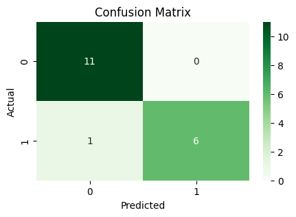
print("Performance Points ")
print(f"Accuracy Point : {acc*100:.2f}")
print(f"Precision Point: {prec*100:.2f}")
print(f"Recall Point : {rec*100:.2f}")
print(f"F1-score Point : {f1*100:.2f}")
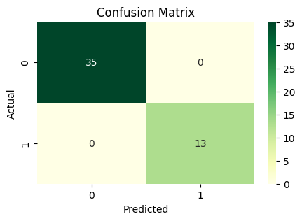
plt.figure(figsize=(5, 3))
sns.heatmap(pd.crosstab(y_test, y_pred), annot=True, fmt="d", cmap="Greens")
plt.xlabel("Predicted")
plt.ylabel("Actual")
plt.title("Confusion Matrix")
plt.show()
Performance Points
Accuracy Point : 94.44
Precision Point: 100.00
Recall Point   : 85.71
F1-score Point : 92.31
import pandas as pd
from sklearn.model_selection import train_test_split
from sklearn.ensemble import RandomForestClassifier
from sklearn.metrics import accuracy_score, classification_report
import seaborn as sns
import matplotlib.pyplot as plt
df = pd.read_csv("heart.csv")
df.columns = df.columns.str.strip().str.upper().str.replace(" ", "_")
df.dropna(inplace=True)
X = df.drop("TARGET", axis=1)
y = df["TARGET"]
X_train, X_test, y_train, y_test = train_test_split(X, y, test_size=0.3, random_state=42)
model = RandomForestClassifier(n_estimators=100, random_state=42)
model.fit(X_train, y_train)
y_pred = model.predict(X_test)
report = classification_report(y_test, y_pred, output_dict=True)
acc = accuracy_score(y_test, y_pred)
prec = report['1']['precision']
rec = report['1']['recall']
f1 = report['1']['f1-score']
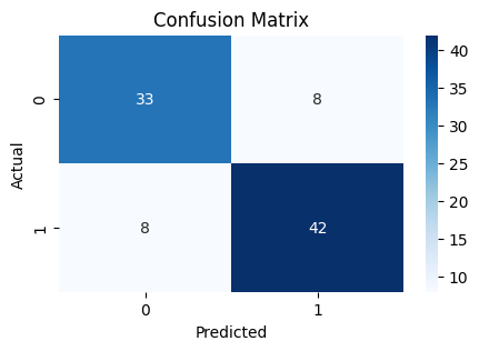
print("Performance Points")
print(f"Accuracy Point : {acc*100:.2f}")
print(f"Precision Point: {prec*100:.2f}")
print(f"Recall Point : {rec*100:.2f}")
print(f"F1-score Point : {f1*100:.2f}")
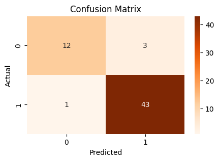
plt.figure(figsize=(5, 3))
sns.heatmap(pd.crosstab(y_test, y_pred), annot=True, fmt="d", cmap="Blues")
plt.xlabel("Predicted")
plt.ylabel("Actual")
plt.title("Confusion Matrix")
plt.show()
Performance Points
Accuracy Point : 82.42
Precision Point: 84.00
Recall Point   : 84.00
F1-score Point : 84.00
import pandas as pd
from sklearn.model_selection import train_test_split
from sklearn.ensemble import RandomForestClassifier
from sklearn.metrics import accuracy_score, classification_report
import seaborn as sns
import matplotlib.pyplot as plt
df = pd.read_csv("diabetes.csv")
df.columns = df.columns.str.strip().str.upper().str.replace(" ", "_")
df.dropna(inplace=True)
X = df.drop("OUTCOME", axis=1)
y = df["OUTCOME"]
X_train, X_test, y_train, y_test = train_test_split(X, y, test_size=0.3, random_state=42)
model = RandomForestClassifier(n_estimators=100, random_state=42)
model.fit(X_train, y_train)
y_pred = model.predict(X_test)
report = classification_report(y_test, y_pred, output_dict=True)
acc = accuracy_score(y_test, y_pred)
prec = report['1']['precision']
rec = report['1']['recall']
f1 = report['1']['f1-score']
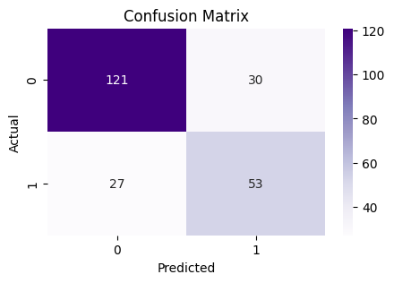
print("Performance Points")
print(f"Accuracy Point : {acc*100:.2f}")
print(f"Precision Point: {prec*100:.2f}")
print(f"Recall Point : {rec*100:.2f}")
print(f"F1-score Point : {f1*100:.2f}")
plt.figure(figsize=(5, 3))
sns.heatmap(pd.crosstab(y_test, y_pred), annot=True, fmt="d", cmap="Purples")
plt.xlabel("Predicted")
plt.ylabel("Actual")
plt.title("Confusion Matrix")
plt.show()
Performance Points
Accuracy Point : 75.32
Precision Point: 63.86
Recall Point   : 66.25
F1-score Point : 65.03
import pandas as pd
from sklearn.model_selection import train_test_split
from sklearn.ensemble import RandomForestClassifier
from sklearn.metrics import accuracy_score, classification_report
import seaborn as sns
import matplotlib.pyplot as plt
df = pd.read_csv("breast_cancer.csv")
df.columns = df.columns.str.strip().str.upper().str.replace(" ", "_")
df['DIAGNOSIS'] = df['DIAGNOSIS'].replace({'M': 1, 'B': 0})
df = df.infer_objects(copy=False)
df.dropna(inplace=True)
X = df.drop(["DIAGNOSIS", "ID"], axis=1, errors='ignore')
y = df["DIAGNOSIS"]
X_train, X_test, y_train, y_test = train_test_split(X, y, test_size=0.3, random_state=42)
model = RandomForestClassifier(n_estimators=100, random_state=42)
model.fit(X_train, y_train)
y_pred = model.predict(X_test)
report = classification_report(y_test, y_pred, output_dict=True)
acc = accuracy_score(y_test, y_pred)
prec = report['1']['precision']
rec = report['1']['recall']
f1 = report['1']['f1-score']
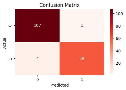
print("Performance Points")
print(f"Accuracy Point : {acc*100:.2f}")
print(f"Precision Point: {prec*100:.2f}")
print(f"Recall Point : {rec*100:.2f}")
print(f"F1-score Point : {f1*100:.2f}")
plt.figure(figsize=(5, 3))
sns.heatmap(pd.crosstab(y_test, y_pred), annot=True, fmt="d", cmap="Reds")
plt.xlabel("Predicted")
plt.ylabel("Actual")
plt.title("Confusion Matrix")
plt.show()
Performance Points
Accuracy Point : 97.08
Precision Point: 98.33
Recall Point   : 93.65
F1-score Point : 95.93
import pandas as pd
from sklearn.model_selection import train_test_split
from sklearn.ensemble import RandomForestClassifier
from sklearn.metrics import accuracy_score, classification_report
import seaborn as sns
import matplotlib.pyplot as plt
df = pd.read_csv("kidney_disease.csv")
df.columns = df.columns.str.strip().str.upper().str.replace(" ", "_")
df.replace({
    'yes': 1, 'no': 0,
    'normal': 0, 'abnormal': 1,
    'present': 1, 'notpresent': 0,
    'ckd': 1, 'notckd': 0,
    'CKD': 1, 'NOTCKD': 0,
    'good': 1, 'poor': 0
}, inplace=True)
df.drop(['ID'], axis=1, errors='ignore', inplace=True)
df.dropna(inplace=True)
df['CLASSIFICATION'] = df['CLASSIFICATION'].astype(int)
X = df.drop("CLASSIFICATION", axis=1)
y = df["CLASSIFICATION"]
X_train, X_test, y_train, y_test = train_test_split(
    X, y, test_size=0.3, random_state=42
)

model = RandomForestClassifier(n_estimators=100, random_state=42)
model.fit(X_train, y_train)
y_pred = model.predict(X_test)
report = classification_report(y_test, y_pred, output_dict=True)
acc = accuracy_score(y_test, y_pred)
prec = report['1']['precision']
rec = report['1']['recall']
f1 = report['1']['f1-score']
print("Performance Points")
print(f"Accuracy Point : {acc*100:.2f}")
print(f"Precision Point: {prec*100:.2f}")
print(f"Recall Point   : {rec*100:.2f}")
print(f"F1-score Point : {f1*100:.2f}")
plt.figure(figsize=(5, 3))
sns.heatmap(pd.crosstab(y_test, y_pred), annot=True, fmt="d", cmap="YlGn")
plt.xlabel("Predicted")
plt.ylabel("Actual")
plt.title("Confusion Matrix")
plt.show()
Performance Points
Accuracy Point : 100.00
Precision Point: 100.00
Recall Point   : 100.00
F1-score Point : 100.00
import pandas as pd
from sklearn.model_selection import train_test_split
from sklearn.ensemble import RandomForestClassifier
from sklearn.metrics import accuracy_score, classification_report
import seaborn as sns
import matplotlib.pyplot as plt
df = pd.read_csv("parkinsons.csv")
df.drop("name", axis=1, inplace=True)
X = df.drop("status", axis=1)   # status = 1 (Parkinson's), 0 (Healthy)
y = df["status"]
X_train, X_test, y_train, y_test = train_test_split(
    X, y, test_size=0.3, random_state=42
)
model = RandomForestClassifier(n_estimators=100, random_state=42)
model.fit(X_train, y_train)
y_pred = model.predict(X_test)
report = classification_report(y_test, y_pred, output_dict=True)
acc = accuracy_score(y_test, y_pred)
prec = report['1']['precision']
rec = report['1']['recall']
f1 = report['1']['f1-score']
print("Performance Points")
print(f"Accuracy Point : {acc*100:.2f}")
print(f"Precision Point: {prec*100:.2f}")
print(f"Recall Point   : {rec*100:.2f}")
print(f"F1-score Point : {f1*100:.2f}")
plt.figure(figsize=(5, 3))
sns.heatmap(pd.crosstab(y_test, y_pred), annot=True, fmt="d", cmap="Oranges")
plt.xlabel("Predicted")
plt.ylabel("Actual")
plt.title("Confusion Matrix")
plt.show()
Performance Points
Accuracy Point : 93.22
Precision Point: 93.48
Recall Point   : 97.73
F1-score Point : 95.56
import pandas as pd
from sklearn.model_selection import train_test_split
from sklearn.ensemble import RandomForestClassifier
from sklearn.metrics import accuracy_score, classification_report
import seaborn as sns
import matplotlib.pyplot as plt
df = pd.read_csv("COVID19_symptoms.csv")
df.columns = df.columns.str.strip().str.upper().str.replace(" ", "_")
df.replace({
'YES': 1, 'NO': 0,
'NONE': 0,
'GOOD': 1, 'POOR': 0,
'FEMALE': 0, 'MALE': 1, 'TRANSGENDER': 2,
"DON'T-KNOW": 2
}, inplace=True)
df.drop(['COUNTRY'], axis=1, inplace=True)
df.dropna(inplace=True)
def encode_severity(row):
if row['SEVERITY_NONE'] == 1:
return 0
elif row['SEVERITY_MILD'] == 1:
return 1
elif row['SEVERITY_MODERATE'] == 1:
return 2
elif row['SEVERITY_SEVERE'] == 1:
return 3
else:
return -1
df['SEVERITY_LABEL'] = df.apply(encode_severity, axis=1)
df.drop(['SEVERITY_NONE', 'SEVERITY_MILD', 'SEVERITY_MODERATE', 'SEVERITY_SEVERE'], axis=1, inplace=True)
X = df.drop("SEVERITY_LABEL", axis=1)
y = df["SEVERITY_LABEL"]
X_train, X_test, y_train, y_test = train_test_split(
X, y, test_size=0.3, random_state=42
)
model = RandomForestClassifier(n_estimators=100, random_state=42)
model.fit(X_train, y_train)
y_pred = model.predict(X_test)
report = classification_report(y_test, y_pred, output_dict=True)
acc = accuracy_score(y_test, y_pred)
print("Performance Metrics")
print(f"Accuracy: {acc*100:.2f}%")
for cls in ["1", "2", "3"]:
if cls in report:
print(f"Class {cls}: Precision {report[cls]['precision']*100:.2f}%, Recall {report[cls]['recall']*100:.2f}%, F1 {report[cls]['f1-score']*100:.2f}%")
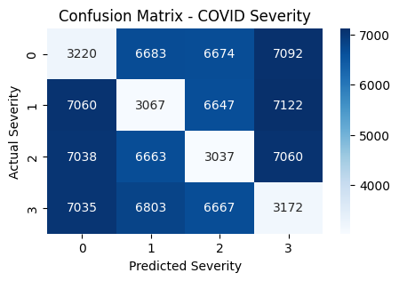
plt.figure(figsize=(5, 3))
sns.heatmap(pd.crosstab(y_test, y_pred), annot=True, fmt="d", cmap="Blues")
plt.xlabel("Predicted Severity")
plt.ylabel("Actual Severity")
plt.title("Confusion Matrix - COVID Severity")
plt.show()
Performance Metrics
Accuracy: 13.15%
Class 1: Precision 13.21%, Recall 12.83%, F1 13.02%
Class 2: Precision 13.19%, Recall 12.76%, F1 12.97%
Class 3: Precision 12.98%, Recall 13.40%, F1 13.18%
import pandas as pd
from sklearn.model_selection import train_test_split
from sklearn.ensemble import RandomForestClassifier
from sklearn.metrics import accuracy_score, classification_report
import seaborn as sns
import matplotlib.pyplot as plt
df = pd.read_csv("survey.csv")
df = df[["Age", "Gender", "family_history", "benefits", "care_options", "seek_help", "mental_health_consequence"]]
df.dropna(inplace=True)
def clean_gender(g):
g = g.lower()
if "male" in g:
return 0
elif "female" in g:
return 1
else:
return 2
df["Gender"] = df["Gender"].apply(clean_gender)
df.replace({
"Yes": 1, "No": 0,
"Don't know": 2, "Not sure": 2, "Maybe": 2,
"Some of them": 1, "Not available": 0
}, inplace=True)
df["mental_health_consequence"] = df["mental_health_consequence"].replace({
"Yes": 1,
"No": 0,
"Maybe": 1 # Treat "Maybe" as potential consequence
})
df["mental_health_consequence"] = df["mental_health_consequence"].astype(int)
X = df.drop("mental_health_consequence", axis=1)
y = df["mental_health_consequence"]
X_train, X_test, y_train, y_test = train_test_split(
X, y, test_size=0.3, random_state=42
)
model = RandomForestClassifier(n_estimators=100, random_state=42)
model.fit(X_train, y_train)
y_pred = model.predict(X_test)
report = classification_report(y_test, y_pred, output_dict=True)
acc = accuracy_score(y_test, y_pred)
print("Mental Health Classification")
print(f"Accuracy : {acc*100:.2f}%")
print(f"Precision (Yes): {report['1']['precision']*100:.2f}%")
print(f"Recall (Yes) : {report['1']['recall']*100:.2f}%")
print(f"F1-score (Yes) : {report['1']['f1-score']*100:.2f}%")
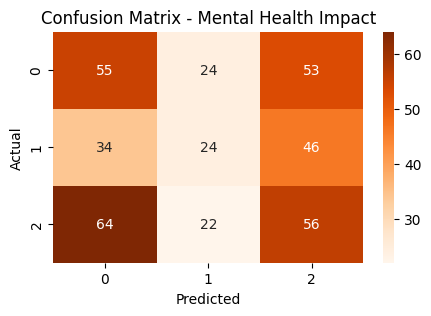
plt.figure(figsize=(5, 3))
sns.heatmap(pd.crosstab(y_test, y_pred), annot=True, fmt="d", cmap="Oranges")
plt.xlabel("Predicted")
plt.ylabel("Actual")
plt.title("Confusion Matrix - Mental Health Impact")
plt.show()
📊 Mental Health Classification
✅ Accuracy       : 35.71%
🎯 Precision (Yes): 34.29%
🔁 Recall (Yes)   : 23.08%
📌 F1-score (Yes) : 27.59%
import pandas as pd
import numpy as np
import matplotlib.pyplot as plt
from sklearn.model_selection import train_test_split
from sklearn.linear_model import LinearRegression
from sklearn.metrics import mean_squared_error, r2_score
df = pd.read_csv("stock_data.csv")
print("Columns in CSV:", df.columns.tolist())
date_col = [col for col in df.columns if 'date' in col.lower() or 'time' in col.lower()]
if date_col:
df[date_col[0]] = pd.to_datetime(df[date_col[0]])
df.set_index(date_col[0], inplace=True)
stock_col = df.select_dtypes(include='number').columns[0]
data = df[[stock_col]].dropna()
data.rename(columns={stock_col: "Close"}, inplace=True)
data["Target"] = data["Close"].shift(-1)
data.dropna(inplace=True)
X = data[["Close"]]
y = data["Target"]
X_train, X_test, y_train, y_test = train_test_split(X, y, test_size=0.2, shuffle=False)
model = LinearRegression()
model.fit(X_train, y_train)
y_pred = model.predict(X_test)
rmse = np.sqrt(mean_squared_error(y_test, y_pred))
r2 = r2_score(y_test, y_pred)
print(f"RMSE: {rmse:.2f}")
print(f"R² Score: {r2:.2f}")
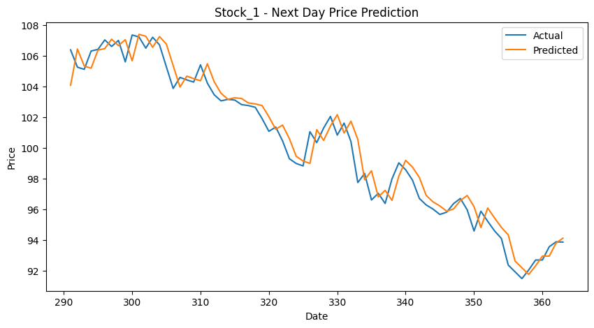
plt.figure(figsize=(10, 5))
plt.plot(y_test.index, y_test, label="Actual")
plt.plot(y_test.index, y_pred, label="Predicted")
plt.title(f"{stock_col} - Next Day Price Prediction")
plt.xlabel("Date")
plt.ylabel("Price")
plt.legend()
plt.show()
Columns in CSV: ['Unnamed: 0', 'Stock_1', 'Stock_2', 'Stock_3', 'Stock_4', 'Stock_5']
RMSE: 0.98
R² Score: 0.96
import pandas as pd
import numpy as np
import matplotlib.pyplot as plt
from sklearn.ensemble import RandomForestRegressor
from sklearn.metrics import mean_squared_error, r2_score
from sklearn.model_selection import train_test_split
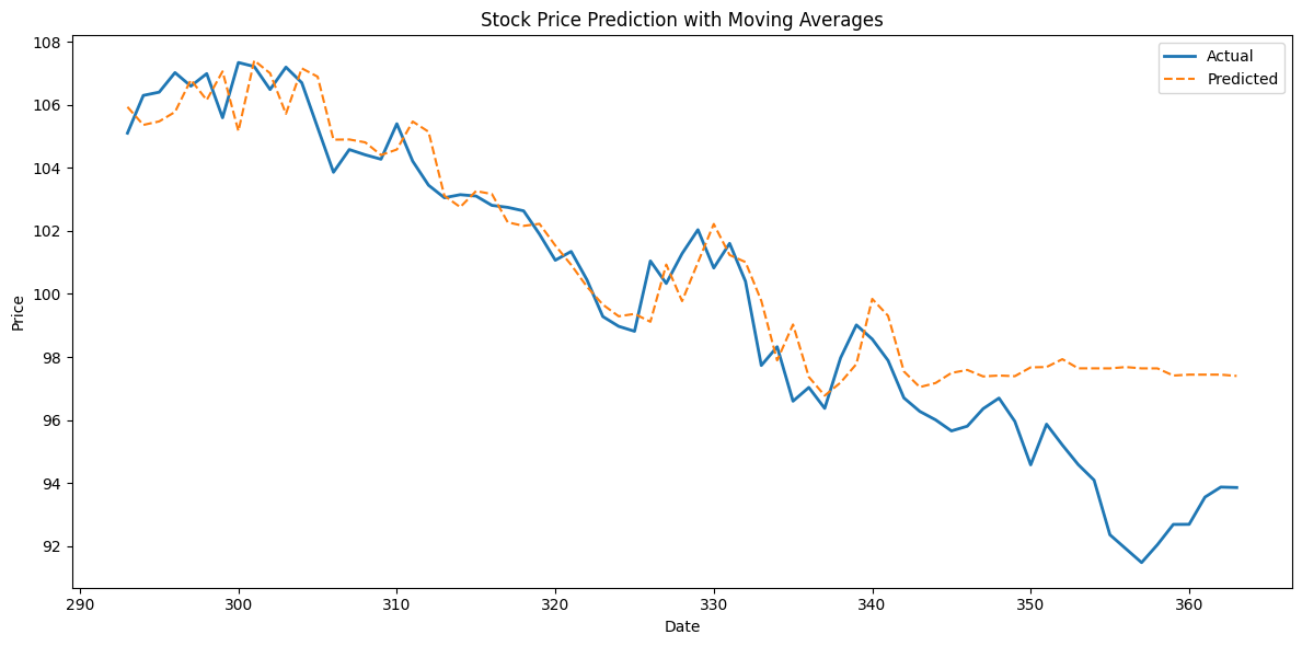
df = pd.read_csv("stock_data.csv")
date_col = [col for col in df.columns if 'date' in col.lower() or 'time' in col.lower()]
if date_col:
df[date_col[0]] = pd.to_datetime(df[date_col[0]])
df.set_index(date_col[0], inplace=True)
stock_col = df.select_dtypes(include='number').columns[0]
df = df[[stock_col]].rename(columns={stock_col: "Close"})
df["MA_5"] = df["Close"].rolling(window=5).mean()
df["MA_10"] = df["Close"].rolling(window=10).mean()
df["Daily_Return"] = df["Close"].pct_change()
df["Target"] = df["Close"].shift(-1) # Predict next day's price
df.dropna(inplace=True)
X = df[["Close", "MA_5", "MA_10", "Daily_Return"]]
y = df["Target"]
X_train, X_test, y_train, y_test = train_test_split(X, y, shuffle=False, test_size=0.2)
model = RandomForestRegressor(n_estimators=100, random_state=42)
model.fit(X_train, y_train)
y_pred = model.predict(X_test)
rmse = np.sqrt(mean_squared_error(y_test, y_pred))
r2 = r2_score(y_test, y_pred)
print(f" RMSE: {rmse:.2f}")
print(f" R² Score: {r2:.2f}")
plt.figure(figsize=(12, 6))
plt.plot(y_test.index, y_test, label="Actual", linewidth=2)
plt.plot(y_test.index, y_pred, label="Predicted", linestyle='--')
plt.title("Stock Price Prediction with Moving Averages")
plt.xlabel("Date")
plt.ylabel("Price")
plt.legend()
plt.tight_layout()
plt.show()
 RMSE: 2.13
 R² Score: 0.79
score = 0
import pandas as pd

data = {
    'city': ['Toronto', 'Montreal', 'Waterloo'],
    'points': [80, 70, 90]
}
df = pd.DataFrame(data)
score += 40
df['code'] = [1, 2, 3]
score += 40
df['points'] = df['points'] + 10
score += 40
from datetime import datetime
def get_age(d):
    d1 = datetime.now()
    months = (d1.year - d.year) * 12 + d1.month - d.month
    year = int(months / 12)
    return year
age = get_age(datetime(1991, 1, 1))
score += 40  # Function logic used
df['status'] = df['points'].apply(lambda x: 'Pass' if x >= 90 else 'Fail')
score += 40
print("Final Score:", score)
print(df)
Final Score: 200
       city  points  code status
0   Toronto      90     1   Pass
1  Montreal      80     2   Fail
2  Waterloo     100     3   Pass
import pandas as pd
data = {
    'name': ['Alice', 'Bob', 'Charlie', 'David'],
    'marks': [85, 67, 90, 74]
}
df = pd.DataFrame(data)
def get_grade(mark):
    if mark >= 90:
        return 'A'
    elif mark >= 80:
        return 'B'
    elif mark >= 70:
        return 'C'
    elif mark >= 60:
        return 'D'
    else:
        return 'F'
df['grade'] = df['marks'].apply(get_grade)
average_mark = df['marks'].mean()
df['result'] = df['marks'].apply(lambda x: 'Pass' if x >= 60 else 'Fail')
print(df)
print("Average Mark:", average_mark)
      name  marks grade result
0    Alice     85     B   Pass
1      Bob     67     D   Pass
2  Charlie     90     A   Pass
3    David     74     C   Pass
Average Mark: 79.0
import pandas as pd
from io import StringIO
from datetime import datetime
csv_data = StringIO("""
name,join_date,salary,position
Alice,2016-08-01,95000,Manager
Bob,2019-07-15,60000,Engineer
Charlie,2014-01-10,120000,Director
David,2021-03-20,45000,Intern
Ella,2018-09-30,70000,Engineer
""")
df = pd.read_csv(csv_data, parse_dates=['join_date'])
today = datetime.today()
df['experience_years'] = df['join_date'].apply(lambda d: (today - d).days // 365)
df['salary_after_tax'] = df['salary'].apply(lambda x: x * 0.82)
def get_level(exp, salary):
    if exp >= 8 and salary > 100000:
        return 'Senior Executive'
    elif exp >= 5:
        return 'Experienced'
    elif exp >= 2:
        return 'Mid-Level'
    else:
        return 'Junior'
df['level'] = df.apply(lambda row: get_level(row['experience_years'], row['salary']), axis=1)
high_performers = df[(df['salary'] > 70000) & (df['experience_years'] > 3)]
print("All Employees:\n", df, "\n")
print("High Performers:\n", high_performers)
All Employees:
       name  join_date  salary  position  experience_years  salary_after_tax  \
0    Alice 2016-08-01   95000   Manager                 8           77900.0
1      Bob 2019-07-15   60000  Engineer                 5           49200.0
2  Charlie 2014-01-10  120000  Director                11           98400.0
3    David 2021-03-20   45000    Intern                 4           36900.0
4     Ella 2018-09-30   70000  Engineer                 6           57400.0

              level
0       Experienced
1       Experienced
2  Senior Executive
3         Mid-Level
4       Experienced

High Performers:
       name  join_date  salary  position  experience_years  salary_after_tax  \
0    Alice 2016-08-01   95000   Manager                 8           77900.0
2  Charlie 2014-01-10  120000  Director                11           98400.0

              level
0       Experienced
2  Senior Executive
import pandas as pd
from datetime import datetime
employees = pd.DataFrame({
    'emp_id': [101, 102, 103, 104, 105, 106],
    'name': ['Alice', 'Bob', 'Charlie', 'David', 'Eva', 'Frank'],
    'department': ['Engineering', 'Engineering', 'HR', 'Finance', 'Finance', 'Engineering'],
    'join_date': pd.to_datetime(['2015-05-21', '2018-03-15', '2012-06-30', '2019-01-01', '2017-11-23', '2022-05-19']),
    'salary': [90000, 72000, 60000, 65000, 58000, 50000]
})
projects = pd.DataFrame({
    'project_id': [1, 2, 3, 4],
    'project_name': ['Alpha', 'Beta', 'Gamma', 'Delta'],
    'assigned_to': [[101, 102], [104], [103, 105], [101, 106]],
    'deadline': pd.to_datetime(['2025-12-01', '2024-11-01', '2025-03-15', '2025-08-30'])
})
project_long = projects.explode('assigned_to').rename(columns={'assigned_to': 'emp_id'})
merged = pd.merge(project_long, employees, on='emp_id', how='left')
today = pd.to_datetime(datetime.today().date())
merged['experience_yrs'] = (today - merged['join_date']).dt.days // 365
workload = merged.groupby('emp_id').size().reset_index(name='project_count')
merged = pd.merge(merged, workload, on='emp_id', how='left')
import numpy as np
conditions = [
    (merged['project_count'] >= 3),
    (merged['project_count'] == 2),
    (merged['project_count'] == 1)
]
choices = ['Overloaded', 'Balanced', 'Light']
merged['workload_status'] = np.select(conditions, choices, default='Unassigned')
department_summary = merged.groupby('department').agg(
    total_employees=('emp_id', 'nunique'),
    avg_salary=('salary', 'mean'),
    total_projects=('project_id', 'nunique'),
    avg_experience=('experience_yrs', 'mean')
).reset_index()
top_employees = merged.sort_values('experience_yrs', ascending=False).drop_duplicates('department')
print("\nFull Merged Data (Project Assignments + Employees):")
print(merged[['emp_id', 'name', 'department', 'project_name', 'workload_status', 'experience_yrs']])
print("\nDepartment Summary:")
print(department_summary)
print("\nTop Experienced Employee per Department:")
print(top_employees[['department', 'name', 'experience_yrs', 'salary']])
Full Merged Data (Project Assignments + Employees):
  emp_id     name   department project_name workload_status  experience_yrs
0    101    Alice  Engineering        Alpha        Balanced              10
1    102      Bob  Engineering        Alpha           Light               7
2    104    David      Finance         Beta           Light               6
3    103  Charlie           HR        Gamma           Light              13
4    105      Eva      Finance        Gamma           Light               7
5    101    Alice  Engineering        Delta        Balanced              10
6    106    Frank  Engineering        Delta           Light               3

Department Summary:
    department  total_employees  avg_salary  total_projects  avg_experience
0  Engineering                3     75500.0               2             7.5
1      Finance                2     61500.0               2             6.5
2           HR                1     60000.0               1            13.0

Top Experienced Employee per Department:
    department     name  experience_yrs  salary
3           HR  Charlie              13   60000
5  Engineering    Alice              10   90000
4      Finance      Eva               7   58000
import pandas as pd
import numpy as np
from datetime import datetime

# Employee DataFrame
df_emp = pd.DataFrame({
    'emp_id': range(1001, 1031),
    'name': [f'Emp{i}' for i in range(1, 31)],
    'department': np.random.choice(['HR', 'Finance', 'Engineering', 'Sales'], 30),
    'join_date': pd.date_range(start='2010-01-01', periods=30, freq='180D'),
    'salary': np.random.randint(50000, 120000, 30),
    'monthly_sales': np.random.randint(3000, 10000, 30)
})

# Project DataFrame
df_proj = pd.DataFrame({
    'project_id': range(201, 211),
    'project_name': [f'Proj{i}' for i in range(1, 11)],
    'assigned_to': [list(np.random.choice(df_emp['emp_id'], size=np.random.randint(2, 6), replace=False)) for _ in range(10)],
    'deadline': pd.date_range(start='2025-01-01', periods=10, freq='30D')
})

# Enrichment
today = pd.to_datetime(datetime.today().date())
df_emp['experience_years'] = (today - df_emp['join_date']).dt.days // 365
df_emp['tax'] = df_emp['salary'] * 0.18
df_emp['net_salary'] = df_emp['salary'] - df_emp['tax']

# Bonus and performance
def calc_bonus(s): return 0.1 if s >= 9000 else 0.08 if s >= 7000 else 0.05 if s >= 5000 else 0.03
df_emp['bonus_percent'] = df_emp['monthly_sales'].apply(calc_bonus)
df_emp['monthly_bonus'] = df_emp['salary'] * df_emp['bonus_percent']

def perf(s): return 'Excellent' if s >= 9500 else 'Good' if s >= 7000 else 'Average' if s >= 5000 else 'Low'
df_emp['performance'] = df_emp['monthly_sales'].apply(perf)

df_emp['annual_total'] = (df_emp['net_salary'] + df_emp['monthly_bonus']) * 12

def grade(row):
    if row['performance'] == 'Excellent' and row['experience_years'] > 5: return 'A+'
    if row['performance'] == 'Good': return 'A'
    if row['performance'] == 'Average': return 'B'
    return 'C'
df_emp['grade'] = df_emp.apply(grade, axis=1)

df_summary = df_emp.groupby('department').agg(
    avg_salary=('salary', 'mean'),
    max_bonus=('monthly_bonus', 'max'),
    avg_exp=('experience_years', 'mean'),
    perf_score=('performance', lambda x: (x == 'Excellent').sum())
).reset_index()

df_emp['exp_category'] = pd.cut(df_emp['experience_years'], [0, 3, 6, 10, 20], labels=['Junior', 'Mid', 'Senior', 'Veteran'])
df_emp['promotion_eligible'] = (df_emp['experience_years'] >= 5) & (df_emp['performance'].isin(['Excellent', 'Good']))
df_emp['tax_saved'] = df_emp['monthly_bonus'] * 0.3

df_masked = df_emp.copy()
df_masked['tax'] = '****'

df_emp['salary_lakh'] = df_emp['salary'] / 1e5
df_emp['net_salary_lakh'] = df_emp['net_salary'] / 1e5

df_rank = df_emp.groupby('department')['monthly_sales'].mean().rank(ascending=False).astype(int).reset_index()
df_rank.columns = ['department', 'dept_rank']
df_emp = df_emp.merge(df_rank, on='department', how='left')

df_emp['salary_bucket'] = pd.cut(df_emp['salary'], [0, 60000, 80000, 100000, 150000], labels=['<60K', '60-80K', '80-100K', '100K+'])

df_emp['new_salary'] = np.where(df_emp['promotion_eligible'], df_emp['salary'] * 1.1, df_emp['salary'])
score_map = {'Excellent': 3, 'Good': 2, 'Average': 1, 'Low': 0}
df_emp['perf_score'] = df_emp['performance'].map(score_map)
df_emp['sales_z'] = (df_emp['monthly_sales'] - df_emp['monthly_sales'].mean()) / df_emp['monthly_sales'].std()

project_exp = df_proj.explode('assigned_to').rename(columns={'assigned_to': 'emp_id'})
df_merged = project_exp.merge(df_emp, on='emp_id', how='left')

df_merged['days_to_deadline'] = (df_merged['deadline'] - today).dt.days
df_merged['proj_bonus_share'] = df_merged['monthly_bonus'] / df_merged.groupby('project_id')['monthly_bonus'].transform('sum')

df_dept_perf = df_merged.groupby(['department', 'project_name']).agg(
    avg_perf_score=('perf_score', 'mean'),
    total_proj_bonus=('proj_bonus_share', 'sum')
).reset_index()

df_eng = df_emp[df_emp['department'] == 'Engineering'].copy()
df_fin = df_emp[df_emp['department'] == 'Finance'].copy()
df_hr = df_emp[df_emp['department'] == 'HR'].copy()
df_sales = df_emp[df_emp['department'] == 'Sales'].copy()

df_eng.loc[:, 'bench_status'] = np.where(df_eng['monthly_sales'] < 4000, 'Bench', 'Active')
df_fin.loc[:, 'risk'] = np.where(df_fin['experience_years'] < 2, 'High', 'Normal')

df_combined = pd.concat([df_eng, df_fin, df_hr, df_sales])
df_combined['normalized_bonus'] = (df_combined['monthly_bonus'] - df_combined['monthly_bonus'].min()) / (df_combined['monthly_bonus'].max() - df_combined['monthly_bonus'].min())

df_top_perf = df_emp[df_emp['performance'] == 'Excellent'].sort_values('monthly_sales', ascending=False).head(10)
df_low_perf = df_emp[df_emp['performance'] == 'Low'].sort_values('monthly_sales').head(10)

df_proj_perf = df_merged.groupby('project_id').agg(
    avg_sales=('monthly_sales', 'mean'),
    total_employees=('emp_id', 'nunique')
).reset_index()

df_emp['salary_growth'] = df_emp['new_salary'] - df_emp['salary']
df_emp['effective_tax_rate'] = df_emp['tax'] / df_emp['salary']
df_emp['bonus_efficiency'] = df_emp['monthly_bonus'] / df_emp['monthly_sales']
df_emp['net_to_gross_ratio'] = df_emp['net_salary'] / df_emp['salary']

df_perf_deviation = df_emp[['emp_id', 'monthly_sales', 'sales_z']].sort_values('sales_z', ascending=False)
df_bonus_outliers = df_emp[df_emp['monthly_bonus'] > df_emp['monthly_bonus'].mean() + 2 * df_emp['monthly_bonus'].std()]
df_tax_outliers = df_emp[df_emp['tax'] > df_emp['tax'].mean() + 2 * df_emp['tax'].std()]
df_exp_leaders = df_emp.sort_values('experience_years', ascending=False).head(5)
df_newcomers = df_emp.sort_values('join_date', ascending=False).head(5)
df_veterans = df_emp[df_emp['experience_years'] >= 10]

df_emp['efficiency_score'] = df_emp['net_salary'] / (1 + df_emp['experience_years']) * df_emp['bonus_percent']
df_emp['team_fit_score'] = np.where(df_emp['grade'].isin(['A+', 'A']), 1, 0.5)

df_pivot_perf = pd.pivot_table(df_emp, index='department', columns='grade', values='salary', aggfunc='mean').fillna(0)
df_pivot_bonus = pd.pivot_table(df_emp, index='exp_category', columns='performance', values='monthly_bonus', aggfunc='mean', observed=False).fillna(0)

df_proj_long = df_proj.explode('assigned_to').rename(columns={'assigned_to': 'emp_id'})
df_proj_long = df_proj_long.merge(df_emp[['emp_id', 'salary']], on='emp_id', how='left')
df_proj_long['share_salary'] = df_proj_long['salary'] / df_proj_long.groupby('project_id')['salary'].transform('sum')

df_final_export = df_emp[['emp_id', 'name', 'department', 'grade', 'performance', 'monthly_bonus', 'new_salary', 'promotion_eligible']]
df_export_summary = df_emp.groupby('department')[['salary', 'monthly_bonus', 'net_salary']].mean().reset_index()

df_stat = df_emp.describe()
df_exp_group = df_emp.groupby('exp_category', observed=False)[['salary', 'monthly_bonus']].mean().reset_index()
df_ranked = df_emp.sort_values(['perf_score', 'experience_years'], ascending=[False, False])
df_department_max_bonus = df_emp.groupby('department')['monthly_bonus'].max().reset_index()
df_top10_salary = df_emp.sort_values('salary', ascending=False).head(10)
df_bottom10_salary = df_emp.sort_values('salary').head(10)

df_emp['relative_perf'] = df_emp['perf_score'] / df_emp['experience_years'].replace(0, 1)

df_proj_assignments = df_proj_long.groupby('emp_id').agg(total_projects=('project_id', 'count')).reset_index()
df_merged_final = df_emp.merge(df_proj_assignments, on='emp_id', how='left')
df_merged_final['total_projects'] = df_merged_final['total_projects'].fillna(0).astype(int)

df_emp['loyalty_index'] = df_emp['experience_years'] / df_emp['department'].map(df_emp.groupby('department')['experience_years'].mean())
print("\nFinal Employee Data Sample:")
print(df_emp.head())

print("\nDepartment Summary:")
print(df_summary)

print("\nTop 5 Performers:")
print(df_top_perf[['emp_id', 'name', 'monthly_sales', 'performance']])

print("\nNewcomers (Recently Joined):")
print(df_newcomers[['emp_id', 'name', 'join_date']])

print("\nMax Monthly Bonus by Department:")
print(df_department_max_bonus)

print("\nEmployee Stats Description:")
print(df_stat)

print("\nBottom 5 Performers (Low):")
print(df_low_perf[['emp_id', 'name', 'monthly_sales', 'performance']])

print("\nProject Performance Summary:")
print(df_proj_perf)

print("\nExperience Group Summary:")
print(df_exp_group)
Final Employee Data Sample:
   emp_id  name   department  join_date  salary  monthly_sales  \
0    1001  Emp1        Sales 2010-01-01   79408           9961
1    1002  Emp2           HR 2010-06-30  110847           8478
2    1003  Emp3      Finance 2010-12-27   55721           9216
3    1004  Emp4           HR 2011-06-25   84660           8227
4    1005  Emp5  Engineering 2011-12-22  101856           6356

   experience_years       tax  net_salary  bonus_percent  ...  perf_score  \
0                15  14293.44    65114.56           0.10  ...           3
1                15  19952.46    90894.54           0.08  ...           2
2                14  10029.78    45691.22           0.10  ...           2
3                14  15238.80    69421.20           0.08  ...           2
4                13  18334.08    83521.92           0.05  ...           1

    sales_z  salary_growth effective_tax_rate bonus_efficiency  \
0  2.041904         7940.8               0.18         0.797189
1  1.268971        11084.7               0.18         1.045973
2  1.653613         5572.1               0.18         0.604612
3  1.138151         8466.0               0.18         0.823241
4  0.162995            0.0               0.18         0.801259

   net_to_gross_ratio  efficiency_score  team_fit_score  relative_perf  \
0                0.82        406.966000             1.0       0.200000
1                0.82        454.472700             1.0       0.133333
2                0.82        304.608133             1.0       0.142857
3                0.82        370.246400             1.0       0.142857
4                0.82        298.292571             0.5       0.076923

   loyalty_index
0       1.849315
1       1.849315
2       1.666667
3       1.726027
4       1.750000

[5 rows x 32 columns]

Department Summary:
    department    avg_salary  max_bonus   avg_exp  perf_score
0  Engineering  83046.857143    7752.80  7.428571           2
1      Finance  72508.000000    5572.10  8.400000           0
2           HR  86317.555556    8867.76  8.111111           0
3        Sales  86086.222222    7940.80  8.111111           1

Top 5 Performers:
    emp_id   name  monthly_sales performance
0     1001   Emp1           9961   Excellent
10    1011  Emp11           9908   Excellent
14    1015  Emp15           9589   Excellent

Newcomers (Recently Joined):
    emp_id   name  join_date
29    1030  Emp30 2024-04-17
28    1029  Emp29 2023-10-20
27    1028  Emp28 2023-04-23
26    1027  Emp27 2022-10-25
25    1026  Emp26 2022-04-28

Max Monthly Bonus by Department:
    department  monthly_bonus
0  Engineering        7752.80
1      Finance        5572.10
2           HR        8867.76
3        Sales        7940.80

Employee Stats Description:
            emp_id            join_date         salary  monthly_sales  \
count    30.000000                   30      30.000000      30.000000
mean   1015.500000  2017-02-23 00:00:00   83183.400000    6043.266667
min    1001.000000  2010-01-01 00:00:00   54449.000000    3577.000000
25%    1008.250000  2013-07-29 00:00:00   69237.750000    4554.500000
50%    1015.500000  2017-02-23 00:00:00   84854.500000    5897.000000
75%    1022.750000  2020-09-20 00:00:00   93228.500000    6696.250000
max    1030.000000  2024-04-17 00:00:00  113569.000000    9961.000000
std       8.803408                  NaN   17923.305573    1918.667155

       experience_years           tax   net_salary  bonus_percent  \
count         30.000000     30.000000     30.00000      30.000000
mean           8.000000  14973.012000  68210.38800       0.052333
min            1.000000   9800.820000  44648.18000       0.030000
25%            4.250000  12462.795000  56774.95500       0.030000
50%            8.000000  15273.810000  69580.69000       0.050000
75%           11.750000  16781.130000  76447.37000       0.050000
max           15.000000  20442.420000  93126.58000       0.100000
std            4.394354   3226.195003  14697.11057       0.024167

       monthly_bonus  annual_total  ...  dept_rank     new_salary  perf_score  \
count      30.000000  3.000000e+01  ...  30.000000      30.000000   30.000000
mean     4320.721667  8.703733e+05  ...   2.666667   84784.186667    0.966667
min      1735.470000  5.684476e+05  ...   1.000000   54449.000000    0.000000
25%      2751.517500  7.062251e+05  ...   2.000000   69237.750000    0.000000
50%      3554.600000  9.011198e+05  ...   3.000000   87755.400000    1.000000
75%      5556.537500  9.544479e+05  ...   4.000000   93289.500000    1.000000
max      8867.760000  1.197148e+06  ...   4.000000  121931.700000    3.000000
std      2061.872362  1.872966e+05  ...   1.154701   18255.231495    0.964305

            sales_z  salary_growth  effective_tax_rate  bonus_efficiency  \
count  3.000000e+01      30.000000        3.000000e+01         30.000000
mean   1.202742e-16    1600.786667        1.800000e-01          0.695374
min   -1.285406e+00       0.000000        1.800000e-01          0.427559
25%   -7.759380e-01       0.000000        1.800000e-01          0.539667
50%   -7.623348e-02       0.000000        1.800000e-01          0.672981
75%    3.403317e-01       0.000000        1.800000e-01          0.800241
max    2.041904e+00   11084.700000        1.800000e-01          1.056824
std    1.000000e+00    3341.600041        2.775558e-17          0.188540

       net_to_gross_ratio  efficiency_score  team_fit_score
count        3.000000e+01         30.000000       30.000000
mean         8.200000e-01        521.664180        0.616667
min          8.200000e-01        166.211071        0.500000
25%          8.200000e-01        255.058950        0.500000
50%          8.200000e-01        379.230183        0.500000
75%          8.200000e-01        587.154850        0.500000
max          8.200000e-01       2259.038500        1.000000
std          8.246530e-17        451.629510        0.215092

[8 rows x 23 columns]

Bottom 5 Performers (Low):
    emp_id   name  monthly_sales performance
24    1025  Emp25           3577         Low
20    1021  Emp21           3725         Low
7     1008   Emp8           3733         Low
18    1019  Emp19           3910         Low
26    1027  Emp27           4010         Low
19    1020  Emp20           4212         Low
6     1007   Emp7           4291         Low
15    1016  Emp16           4485         Low
27    1028  Emp28           4763         Low
16    1017  Emp17           4794         Low

Project Performance Summary:
   project_id    avg_sales  total_employees
0         201  6093.500000                4
1         202  5978.333333                3
2         203  7732.750000                4
3         204  7503.000000                2
4         205  6583.000000                3
5         206  5374.000000                4
6         207  6820.000000                5
7         208  5728.333333                3
8         209  4523.750000                4
9         210  6219.333333                3

Experience Group Summary:
  exp_category        salary  monthly_bonus
0       Junior  81796.333333     3771.06500
1          Mid  86197.333333     3235.45000
2       Senior  78405.875000     4454.57375
3      Veteran  86029.300000     5194.59700
Score: 35
Category: basics